Reward, Risk, and Win Rate: Understand Trading Expectancy

Define the ratio before using it

This article writes reward:risk in that order. A 2:1 ratio means a proposed reward twice the proposed loss. Some sources reverse the labels, so the numbers alone are ambiguous.

A target ratio describes a proposed trade. Expectancy describes a weighted average outcome under stated assumptions about wins, losses, and costs. An attractive target does not establish how often it will be reached.

The CME risk-management guide introduces the relationship between risk and reward. The calculations below are independent hypothetical examples, not measured results of the course techniques.

Measure target space from the actual structure

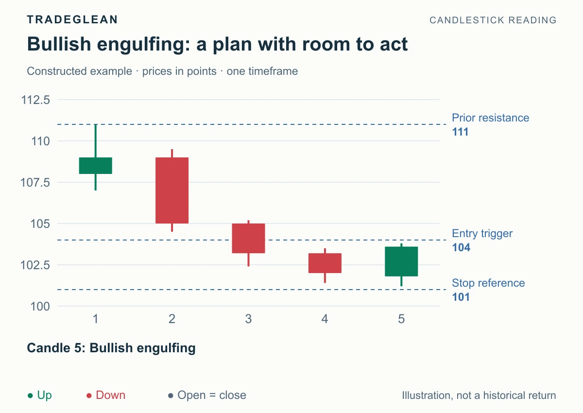
Suppose a linear long position enters at 105, has a protective trigger at 100, and faces resistance at 112. Ignoring costs and slippage, the price risk is 5 points and the available move is 7 points: 7 ÷ 5 = 1.4, or 1.4:1 reward:risk.

Moving the target to 115 makes the arithmetic read 2:1, but does not remove resistance at 112. Tightening the stop to 101.5 also changes the ratio, but might no longer match the setup's failure condition. Let the structure determine the distances before assessing the ratio.

A measured-move projection can provide another reference. It is not evidence that the projected price must trade.

Use R as a fixed reference

1R here is the position's initial planned price loss from entry to protective trigger, in money, before costs. If that amount is 100, a gross gain of 150 is +1.5R and a gross loss of 100 is −1R.

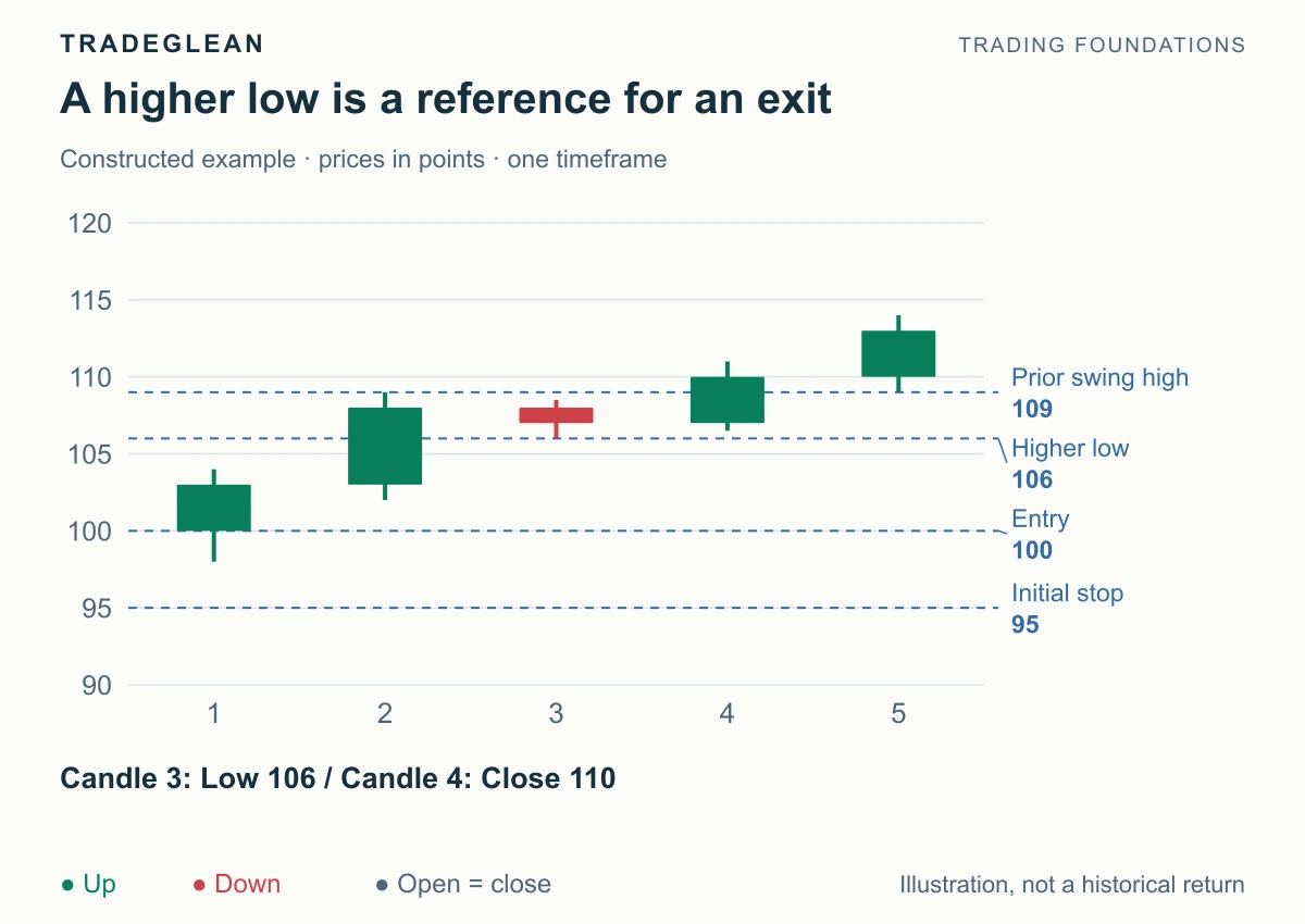
Keep that denominator fixed when comparing possible exits. Moving a stop to the entry does not turn the original 100 risk into zero for the R calculation. A loss beyond the trigger can exceed −1R.

Calculate a weighted average

Let p be the win probability, W the average gross win in R, L the average gross loss magnitude in R, and C the average cost per trade in R:

Expectancy = p × W − (1 − p) × L − C.

Hypothetical outcomes	Before costs	With 0.05R average cost
40% wins; +1.5R wins; −1R losses	0.4 × 1.5 − 0.6 × 1 = 0R	−0.05R
40% wins; +2R wins; −1R losses	0.4 × 2 − 0.6 × 1 = +0.20R	+0.15R
60% wins; +0.5R wins; −1R losses	0.6 × 0.5 − 0.4 × 1 = −0.10R	−0.15R

These rows explain the arithmetic. They do not assign probabilities to any candlestick pattern. In particular, 40% wins at 1.5:1 is break-even before costs under these assumptions, not a profitable edge.

Find the break-even win rate

With constant W, L, and average C under the same model:

Break-even p = (L + C) ÷ (W + L).

For W = 2, L = 1, and C = 0, the result is exactly one-third, about 33.33%. At 33%, expectancy is slightly negative. With C = 0.05, the threshold becomes 35%.

Use net wins and net losses instead if those figures already include fees; do not also subtract C. Trading-cost examples explain this double-counting problem.

Partial exits change the average result

If half a position exits at +2R and half at the entry price, the full position earns +1R gross, not +2R. If losses still average −1R, that changes the win rate needed to break even.

A planned ratio, an assumed win rate, and an illustrative chart cannot prove positive expectancy. Even a positive average under a model can include losing sequences and large individual losses. The calculation also does not describe outcomes accurately when position sizes vary unless the weighting is adjusted.

Compare fixed targets, partial exits, and trailing stops to see how the exit rule changes possible outcomes.